I came across a post on Instagram last week. It had the following message (or something similar):
Oscar-winning film Flow raises adoptions for black cats.
It really caught my attention (yea, I love cats). At first glance, I immediately thought of taking an RDiT (Regression Discontinuity in Time) approach where the running variable is time and threshold is whether or not the observation belongs to the post-movie period. However, adoption is a censored variable, for some cats we observe the true event and for some others, we don’t (e.g., maybe a cat runs away or gets transferred to some other shelter). Hence, it hints at time-to-event modeling. So, I changed the question and decided to attempt to answer the following: > Do black cats experience better adoption process than non-black cats, after the movie Flow?
One implication of “better adoption process” would be to wait less. So, the question maps into do black cats wait less to be adopted compared to non-black cats, after the movie Flow? I asked the ChatGPT about the data which directed me to data from Austin TX
I planned on taking a difference-in-differences approach: Within both black and non-black cats, for pre and post movie period, estimate the days until adoption. Then take the difference within, which leads to difference in days between pre and post period for each black and non-black cats. And then, take the difference in differences. I believe the expression below makes it easier to understand: \((\text{black}_{post} - \text{black}_{pre}) - (\text{non-black}_{post} - \text{non-black}_{pre})\)
For time-to-event modeling, a natural choice is exponential distribution with \(\lambda\), where \(\lambda\) reflects the rate of adoption in our case. In general, one can think of it as average number of events per unit of time. However, since there are censored observations, we end up with two distributions that are assigned to observations. It would be easier if I just give the model specification.
\(\displaystyle \text{Exponential}(\lambda_i)\) if true event observed.
\(\displaystyle \text{Exponential-CCDF}(\lambda_i)\) if true event unobserved.
\(\displaystyle \lambda_i = 1 / \mu_i\)
\(\text{log}(\mu_i) = \alpha_0 + \alpha_{\text{black}} \cdot \text{is\_black}_i + \beta_{\text{post}} \cdot \text{post\_movie}_i + \beta_{\text{inter}} \cdot (\text{post\_movie}_i \cdot \text{is\_black}_i) + f_{\text{time}}(\text{month}_i) + \gamma \cdot \text{time\_trend}\)
Prior distribution for each are normal, while month effects are hierarchical:
\(f_{\text{time}}(\text{month}_i) \sim \text{Normal}(0, \sigma_{\text{month}})\), \(\sigma_{\text{month}} \sim \text{Exponential}(1)\)
I aimed to capture seasonality and trend via time and month terms. On the other hand the interaction term, b_inter, gives the extra shift for the black cats, after the movie. However, instead of attempting to interpret the coefficients, we’ll go with posterior contrasts.
While calculating the posterior contrasts, I averaged over the months that both present before and after the movie (since post-movie period doesn’t include summer time). Here’s how the before-after contrasts look both for black (black line) and non-black (red line) cats.
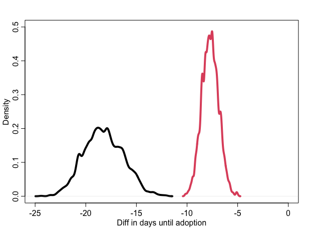
So, it seems like shift for the black cats after the movie is larger compared to non-black cats. 89% HDI for blacks are -21.25 to -18.23 while it’s -9.02 to -7.71 for non-blacks. But, let’s get the difference in differences.
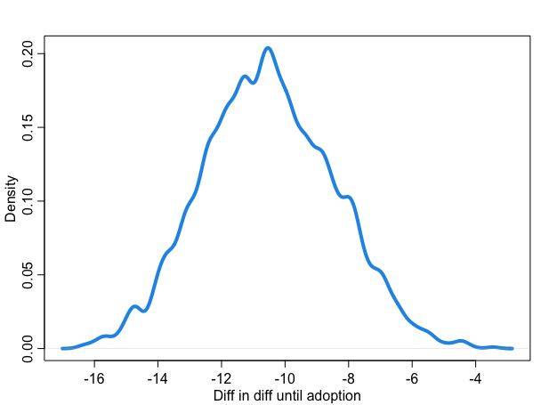
The shift for the black cats after the movie seems to be around 10.5 days. In other words, black cats seem to wait less, after the movie, compared to non-black cats. That’s sweet :)
Alright, to be honest, there’s a caveat here. By modeling it as exponential, I assume that the \(\lambda\) is constant within each strata. There’s no dependence on how long the cat has been waiting. Within a particular stratum, waiting 1 day or 71 days does not make any difference. Well, that’s problematic because that’s unlikely to be true. So, this model can be thought as a baseline and improvements can be make. For example, I thought about swapping to piecewise exponential, where the lambda (the rate) is constant within the day intervals (e.g., 0-7 days, 7-14 days etc.). This might be a next step.
Anyway, I hope you enjoyed this read. See you next time.